The SENSEI User Guide¶

http://hpcvis.com/vis/sensei/rtd-docs/images/write_once.png

SENSEI gives simulations access to a wide array of scalable data analytics and visualization solutions through a single API.

Introduction¶

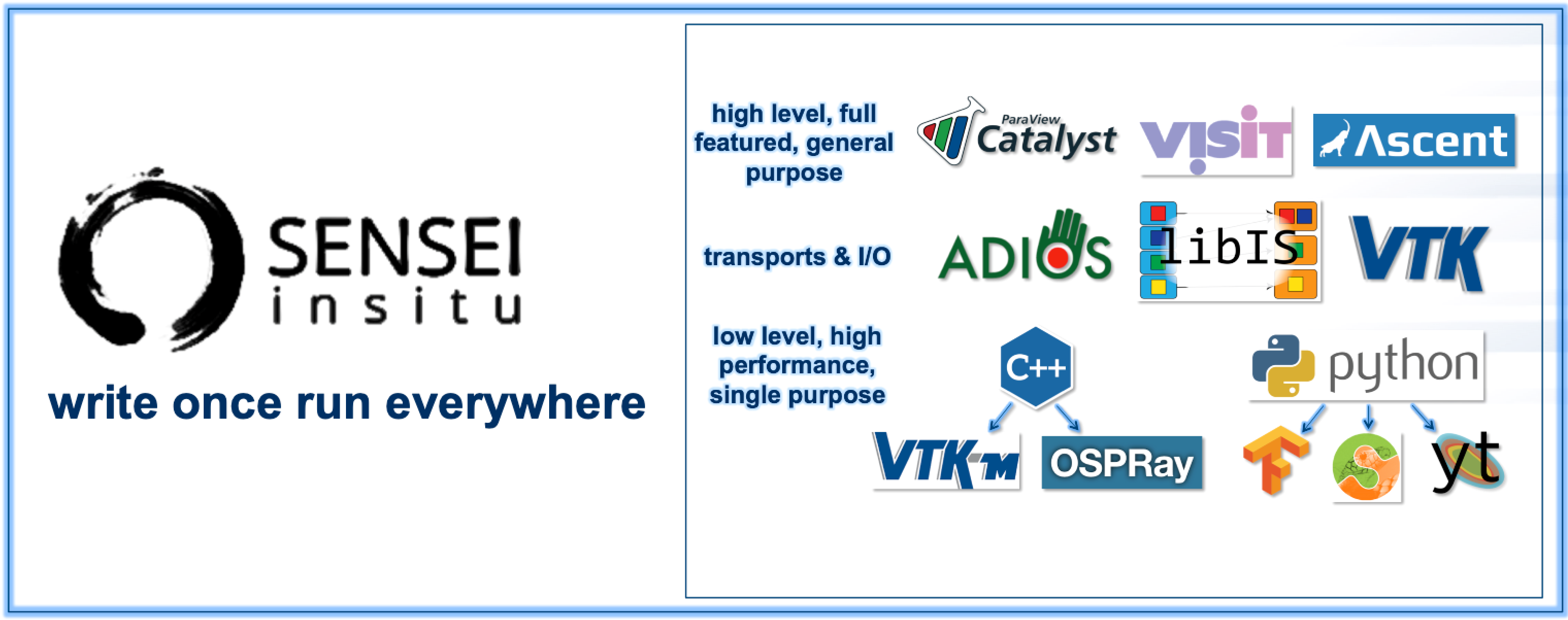
Write once run anywhere. SENSEI seamlessly & efficiently enables in situ data processing with a diverse set of languages, tools & libraries through a simple API, data model, and run-time configuration mechanism.

A SENSEI instrumented simulation can switch between different analysis back-ends such as ADIOS, Libsim, Ascent, Catalyst etc, at run time without modifying code. This flexibility provides options for users, who may have varying needs and preferences about which tools to use to accomplish a task.

Deploying a back end data consumer in SENSEI makes it usable by any SENSEI instrumented simulation. SENSEI is focused on being light weight, having low memory and execution overhead, having a simple API, and minimizing dependencies for each back-end that we support.

Scientists often want to add their own diagnostics in addition to or in place of other back-ends. We strive to make this easy to do in Python and C++. We don’t aim to replace or compete against an individual vis/analysis tool, we aim to make the pie bigger by making their tool and capabilities available to a broader set of users.

With SENSEI the sum is greater than the parts. For instance for both simulations and back-end data consumers, which have not been designed for in transit use, can be run in transit with out modification. Configuring for in transit run makes use of the same simple configuration mechanism that is used to select back-end data consumer.

Write once run everywhere. SENSEI provides access to a diverse set of in situ analysis back-ends and transport layers through a simple API and data model. Simulations instrumented with the SENSEI API can process data using any of these back-ends interchangeably. The back-ends are selected and configured at run-time via an XML configuration file. This document is targeted at scientists and developers wishing to run simulations instrumented with SENSEI, instrument a new simulation, or develop new analysis back-ends.

Source Code¶

SENSEI is open source and freely available on github at https://github.com/SENSEI-insitu/SENSEI.

Online Documentation¶

SENSEI has autmated Doxygen documentation at https://sensei-insitu.readthedocs.io/en/latest/doxygen.

Table of Contents¶

Installation¶

The base install of SENSEI depends on CMake, MPI, Python, SWIG, numpy, and mpi4py.

git clone https://github.com/SENSEI-insitu/SENSEI
mkdir sensei-build
cd sensei-build
cmake ../SENSEI
make -j

This base install enables one to perform in situ in Python using user provided Python scripts. For more information on Python based in situ see our ISAV 2018 paper.

Additional in situ and in transit processing capabilities are available by enabling various build options on the CMake command line.

Build Option	Default	Description
ENABLE_CUDA	OFF	Enables CUDA accelerated codes. Requires compute capability 7.5 and CUDA 11 or later.
ENABLE_PYTHON	ON	Enables Python bindings. Requires Python, Numpy, mpi4py, and SWIG.
ENABLE_CATALYST	OFF	Enables the Catalyst analysis adaptor. Depends on ParaView Catalyst. Set ParaView_DIR.
ENABLE_CATALYST_PYTHON	OFF	Enables Python features of the Catalyst analysis adaptor.
ParaView_DIR		Set to the directory containing ParaViewConfig.cmake.
ENABLE_ASCENT	OFF	Enables the Ascent analysis adaptor. Requires an Ascent install.
ASCENT_DIR		Set to the directory containing the Ascent CMake configuration.
ENABLE_ADIOS2	OFF	Enables ADIOS 2 in transit transport. Set ADIOS2_DIR.
ADIOS2_DIR		Set to the directory containing ADIOSConfig.cmake
ENABLE_HDF5	OFF	Enables HDF5 adaptors and endpoints. Set HDF5_DIR.
HDF5_DIR		Set to the directory containing HDF5Config.cmake
ENABLE_LIBSIM	OFF	Enables Libsim data and analysis adaptors. Requires Libsim. Set VTK_DIR and LIBSIM_DIR.
LIBSIM_DIR		Path to libsim install.
ENABLE_VTK_IO	OFF	Enables adaptors to write to VTK XML format.
ENABLE_VTK_MPI	OFF	Enables MPI parallel VTK filters, such as parallel I/O.
VTK_DIR		Set to the directory containing VTKConfig.cmake.
ENABLE_VTKM	OFF	Enables analyses that use VTK-m. Requires an install of VTK-m. Experimental, each implementation requires an exact version match

System Components¶

System Overview & Architecture¶

SENSEI is a light weight framework for in situ data analysis. SENSEI’s data model and API provide uniform access to and run time selection of a diverse set of visualization and analysis back ends including VisIt Libsim, ParaView Catalyst, VTK-m, Ascent, ADIOS, Yt, and Python.

In situ architecture¶

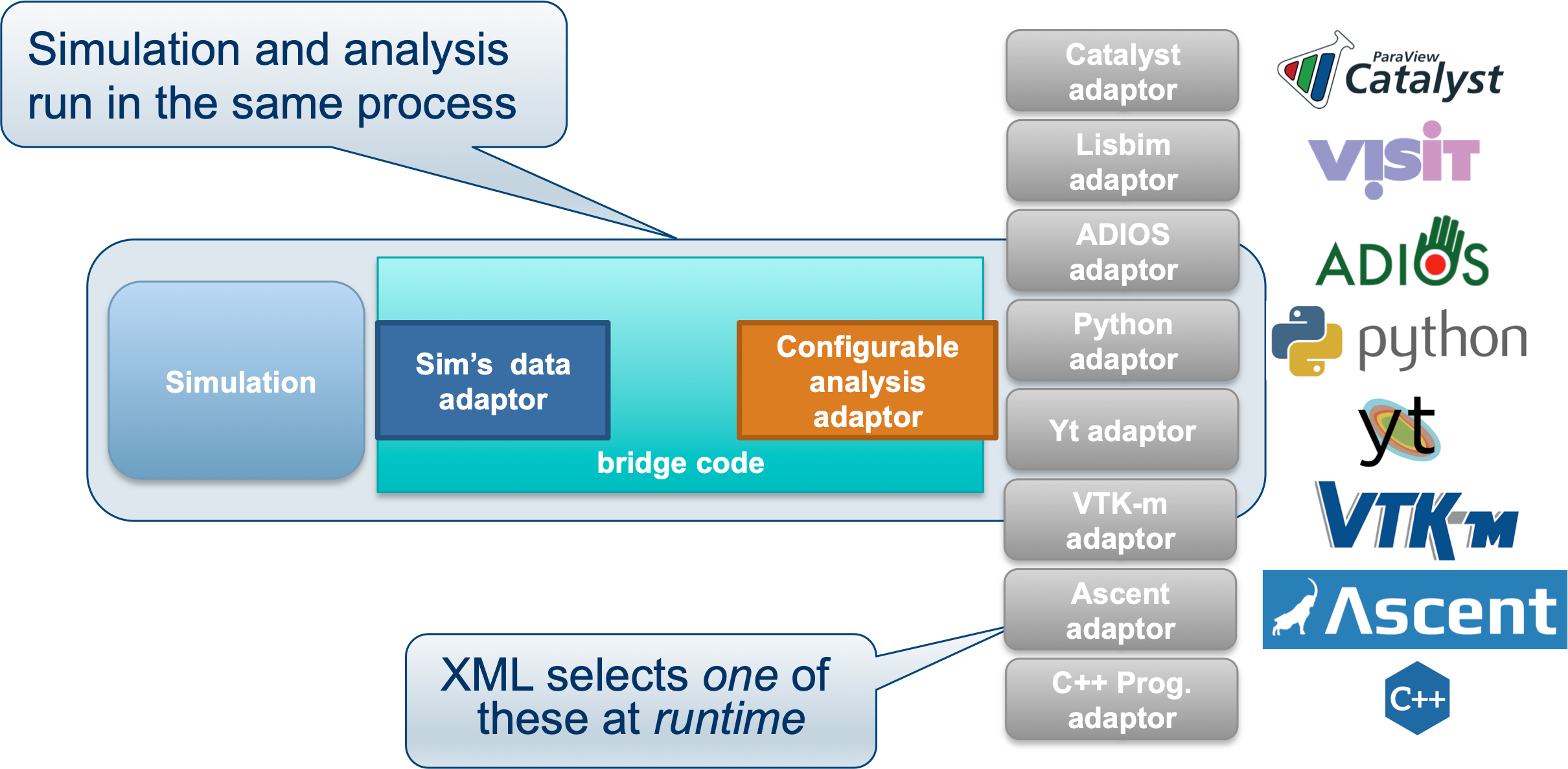
http://hpcvis.com/vis/sensei/rtd-docs/images/sensei_in_situ_arch.png

SENSEI’s in situ architecture enables use of a diverse of back ends which can be selected at run time via an XML configuration file

The three major architectural components in SENSEI are data adaptors which present simulation data in SENSEI’s data model, analysis adaptors which present the back end data consumers to the simulation, and bridge code from which the simulation manages adaptors and periodically pushes data through the system. SENSEI comes equipped with a number of analysis adaptors enabling use of popular analysis and visualization libraries such as VisIt Libsim, ParaView Catalyst, Python, and ADIOS to name a few. AMReX contains SENSEI data adaptors and bridge code making it easy to use in AMReX based simulation codes.

SENSEI provides a configurable analysis adaptor which uses an XML file to select and configure one or more back ends at run time. Run time selection of the back end via XML means one user can access Catalyst, another Libsim, yet another Python with no changes to the code. This is depicted in figure Fig. 2. On the left side of the figure AMReX produces data, the bridge code pushes the data through the configurable analysis adaptor to the back end that was selected at run time.

In transit architecture¶

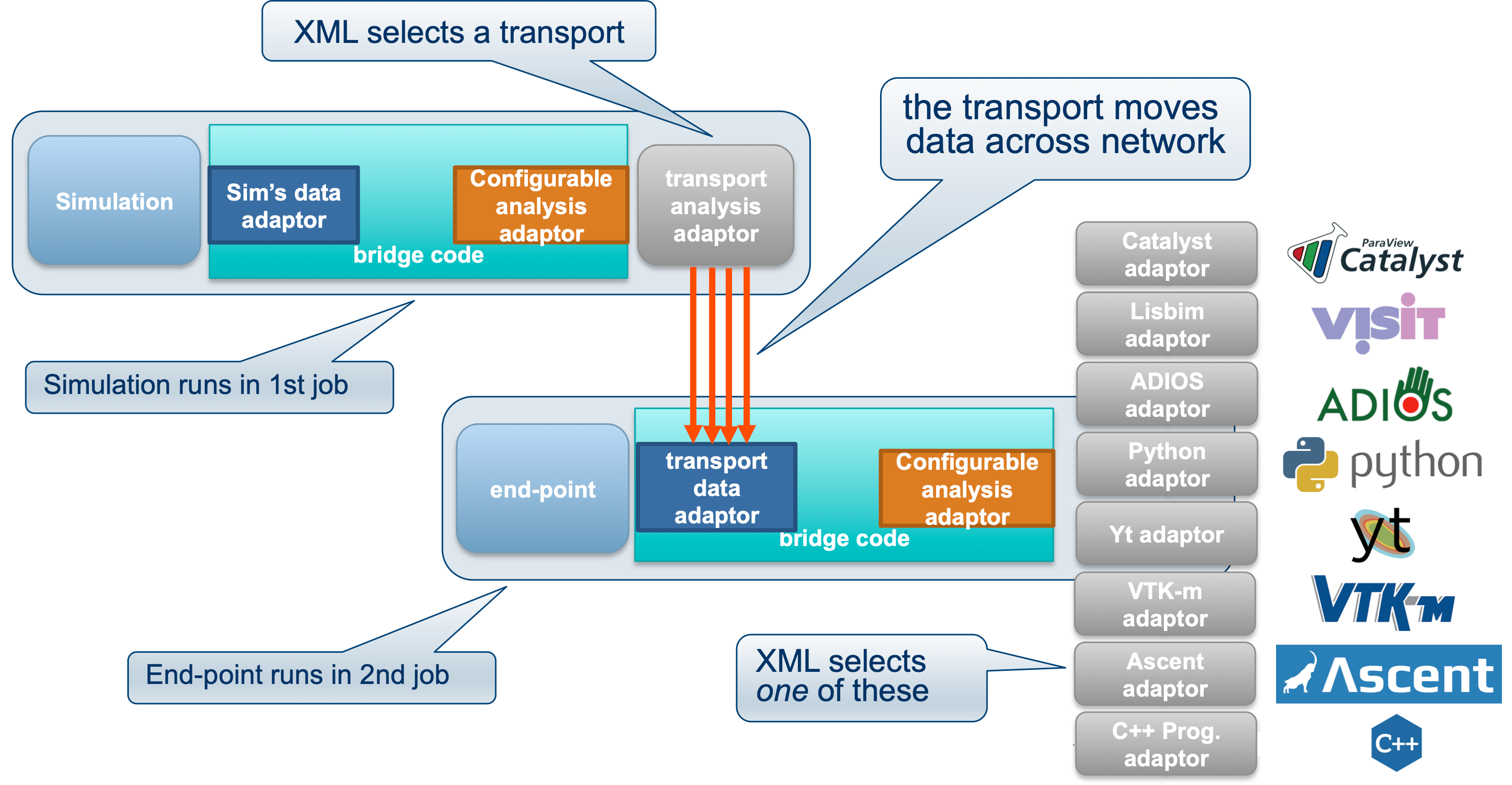
http://hpcvis.com/vis/sensei/rtd-docs/images/sensei_in_transit_arch.png

SENSEI’s in transit architecture enables decoupling of analysis and simulation.

SENSEI’s in transit architecture enables decoupling of analysis and simulation. In this configuration the simulation runs in one job and the analysis runs in a second job, optionally on a separate set of compute resources, optionally at a smaller or larger level of concurrency. The configuration is made possible by a variety of transports who’s job is to move and repartitions data. This is depicted in figure Fig. 3.

In the in transit configuration, the simulation running in one job uses SENSEI’s configurable analysis adaptor to select and configure the write side of the transport. When the simulation pushes data through the SENSEI API for analysis the transport deals with presenting and moving data needed for analysis across the network. In asynchronous mode the simulation proceeds while the data is processed.

A second job, running the SENSEI in transit end-point, uses the configurable analysis adaptor to select and configure one of the back-ends. A transport specific data adaptor presents the available data to the analysis. The analysis can select and request data to be moved across the network for processing.

SENSEI’s design enables this configuration to occur with no changes to either the simulation or analysis back-end. The process is entirely seamless from the simulations point of view and can be so if desired on the analysis side as well. SENSEI supports in transit aware analyses, and provides API’s for yielding control data repartitioning to the analysis.

Adaptor API’s¶

SENSEI makes heavy use of the adaptor design pattern. This pattern is used to abstract away the details of complex and diverse systems exposing them through a single API. SENSEI has 2 types of adaptor. The DataAdaptor abstracts away the details of accessing simulation data. This let’s analysis back-ends access any simulation’s data through a single API. The AnalysisAdaptor abstarcts away the details of the analysis back-ends. This let’s the simulation invoke all of the various analysis back-ends through a single API. When a simulation invokes an analysis back-end it passes it a DataAdaptor that can be used to access simulation data.

DataAdaptor API¶

SENSEI’s data adaptor API abstracts away the differences between simulations allowing SENSEI’s transports and analysis back ends to access data from any simulation in the same way. A simulation must implement the data adaptor API and pass an instance when it wishes to trigger in situ processing.

Through the data adaptor API the analysis back end can get metadata about what the simulation can provide. This metadata is examined and then the analysis can use the API to fetch only the data it needs to accomplish the tasks it has been configured to do.

Finally the data adaptor is a key piece of SENSEI’s in transit system. The analysis back end can be run in a different parallel job and be given an in transit data adaptor in place of the simulation’s data adaptor. In this scenario the in transit data adaptor helps move data needed by the analysis back end. The data adaptor API enables this scenario to apear the same to the simulation and the analysis back end. Neither simulaiton nor analysis need be modified for in transit processing.

Core API¶

Simulations need to implement the core API.

In transit API¶

In transit transports need to implement the in transit API.

AnalysisAdaptor API¶

Show the API in-line, template for writing a new adaptor

Data model¶

The data model is a key piece of the system. It allows data to be packaged and shared between simulations and analysis back ends. SENSEI’s data model relies on VTK’s vtkDataObject class hierarchy to provide containers of array based data, VTK’s conventions for mesh based data (i.e. ordering of FEM cells), and our own metadata object that is used to describe simulation data and it’s mapping onto hardware resources.

Representing mesh based data¶

SENSEI makes use of VTK data object’s to represent simulation data. VTK supports a diverse set of mesh and non-mesh based data. Figure numref:data_types shows a subset of the types of data supported in the VTK data model.

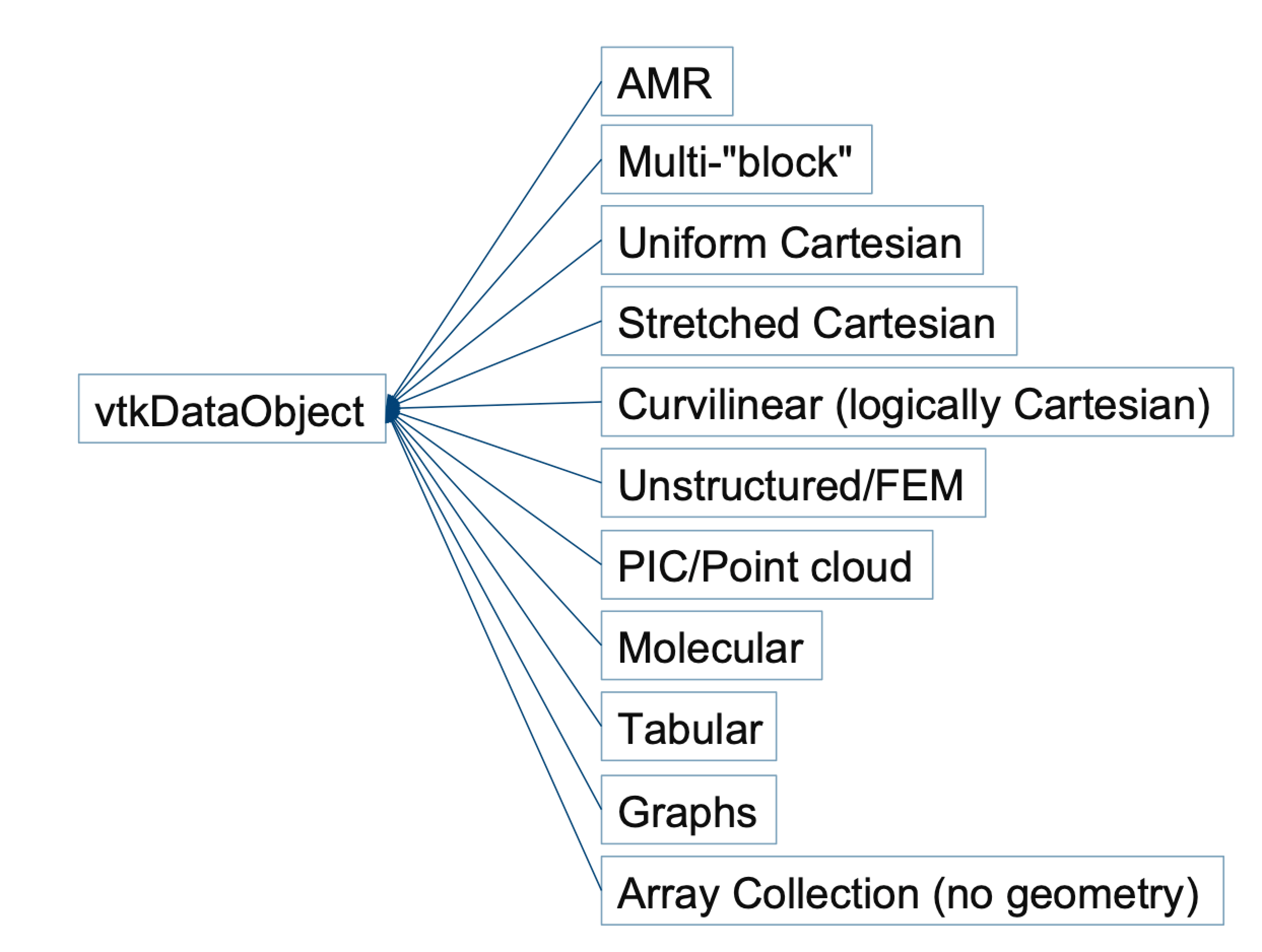
http://hpcvis.com/vis/sensei/rtd-docs/images/data_types.png

A subset of the supported data types.

A key concept in understanding our use of VTK is that we view all data conceptually as multi-block. By multi-block we mean that each MPI rank has zero or more blocks of data. When we say blocks we really mean chunks or pieces, because the blocks can be anything ranging from point sets, to FEM cells, to hierarchical AMR data. to tables, to arrays. The blocks of a multi-block are distributed across the simulation’s MPI ranks with each rank owning a subset of the blocks. An example is depicted in figure numref:multi_block where the 2 data blocks of a multi-block dataset are partitioned across 2 MPI ranks.

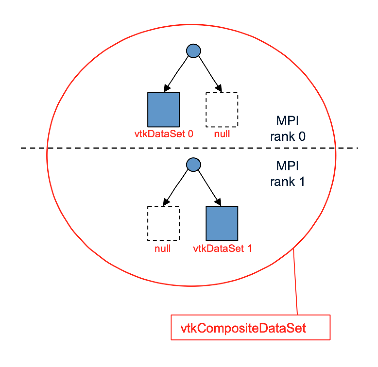
http://hpcvis.com/vis/sensei/rtd-docs/images/multi_block.png

Multi-block data. Each rank has zero or more data blocks. In VTK non-local blocks are nullptr’s.

A strength of VTK is the diversity of data sets that can be represented. A challenge that comes with this lies in VTK’s complexity. SENSEI’s data model only relies on VTK’s common, core and data libraries reducing surface area and complexity when dealing with VTK. While it is possible to use any class derived from vtkDataObject with SENSEI the following data sets are supported universally by all transports and analysis back-ends.

VTK Class	Description
vtkImageData	Blocks of uniform Cartesian geometry
vtkRectilinearGrid	Blocks of stretched Cartesian geometry
vtkUnstructuredGrid	Blocks of finite element method cell zoo and particle meshes
vtkPolyData	Blocks of particle meshes
vtkStructuredGrid	Blocks of logically Cartesian (aka Curvilinear) geometries
vtkOverlappingAMR	A collection of blocks in a block structured AMR hierarchy
vtkMultiBlockDataSet	A collection of data blocks distributed across MPI ranks

As mentioned VTK’s data model is both rich and complex. VTK’s capabilities go well beyond SENSEI’s universal support. However, any dataset type derived from vtkDataObject can be used with SENSEI including those not listed in the table above. The successful use of classes not listed in the above table depends on support implemented by the back end or transport in question.

Representing array based data¶

Each block of a simulation mesh is expected to contain one or more data arrays that hold scalar, vector, and tensor fields generated by the simulation. VTK’s data arrays are used to present array based data. VTK’s data arrays are similar to the STL’s std::vector, but optimized for high-performance computing. One such optimization is the support for zero-copy data transfer. With zero-copy data transfer it is possible to pass a pointer to simulation data directly to an analysis back-end without making a copy of the data.

All of the mesh based types in VTK are derived from vtkDataSet. vtkDataSet defines the common API’s for accessing collections of VTK data arrays by geometric centering. SENSEI supports the following two containers in all back-ends and transports.

Class	Description
vtkPointData	Container of node centered arrays
vtkCellData	Container of cell centered arrays

VTK data arrays support use of any C++ POD type. The two main classes of VTK data arrays of interest here are:

Class	Description
vtkAOSDataArrayTemplate	Use with scalar, vector and tensor data in AOS layout
vtkSOADataArrayTemplate	Use with vector and tensor data in SOA layout

These classes define the API for array based data in VTK. Note the AOS layout is the default in VTK and that classes such as vtkFloatArray, vtkDoubleArray, vtkIntArray etc are aliases to vtkAOSDataArrayTemplate. For simplicity sake one can and should use these aliases anywhere an AOS layout is needed.

Zero-copy into VTK¶

The following snippet of code shows how to pass a 3 component vector field in the AOS layout from the simulation into VTK using the zero-copy mechanism:

// VTK's default is AOS, no need to use vtkAOSDataArrayTemplate
vtkDoubleArray *aos = vtkDoubleArray::New();
aos->SetNumberOfComponents(3);
aos->SetArray(v, 3*nxy, 0);
aos->SetName("velocity");

// add the array as usual
im->GetPointData()->AddArray(aos);

// give up our reference
aos->Delete();

The following snippet of code shows how to pass a 3 component vector field in the SOA layout from the simulation into VTK using the zero-copy mechanism:

// use the SOA class
vtkSOADataArrayTemplate<double> *soa = vtkSOADataArrayTemplate<double>::New();
soa->SetNumberOfComponents(3);

// pass a pointer for each array
soa->SetArray(0, vx, nxy, true);
soa->SetArray(1, vy, nxy);
soa->SetArray(2, vz, nxy);
soa->SetName("velocity");

// add to the image as usual
im->GetPointData()->AddArray(soa);

// git rid of our reference
soa->Delete();

In both these examples ‘im’ is a dataset for some block in a multiblock data set.

Accessing blocks of data¶

This section pertains to accessing data for analysis. During analysis one may obtain a mesh from the simulation. With the mesh in hand one can walk the blocks of data and access the array collections. Arrays in the array collection are accessed and a pointer to the data is obtained for processing. The collections of blocks in VTK are derived from vtkCompositeDataSet. vtkCompositeDataSet defines the API for generically access blocks via the vtkCompositeDataIterator class. The vtkCompositeDataIterator is used to visit all data blocks local to the MPI rank.

Getting help with VTK¶

For those new to VTK a good place to start is the VTK user guide which contains a chapter devoted to learning VTK data model as well as numerous examples. On the VTK community support forums volunteers, and often the VTK developers them selves, answer questions in an effort to help new users.

Metadata¶

SENSEI makes use of a custom metadata object to describe simulation data and its mapping onto hardware resources. This is in large part to support in transit operation where one must make decisions about how simulation data maps onto available analysis resources prior to accessing the data.

Applies to	Field name	Purpose
entire mesh	GlobalView	tells if the information describes data on this rank or all ranks
	MeshName	name of mesh
	MeshType	VTK type enum of the container mesh type
	BlockType	VTK type enum of block mesh type
	NumBlocks	global number of blocks
	NumBlocksLocal	number of blocks on each rank
	Extent	global index space extent \(^{\dagger,\S,*}\)
	Bounds	global bounding box \(^*\)
	CoordinateType	type enum of point data \(^\ddagger\)
	NumPoints	total number of points in all blocks \(^*\)
	NumCells	total number of cells in all blocks \(^*\)
	CellArraySize	total cell array size in all blocks \(^*\)
	NumArrays	number of arrays
	NumGhostCells	number of ghost cell layers
	NumGhostNodes	number of ghost node layers
	NumLevels	number of AMR levels (AMR)
	PeriodicBoundary	indicates presence of a periodic boundary
	StaticMesh	non zero if the mesh does not change in time
each array	ArrayName	name of each data array
	ArrayCentering	centering of each data array
	ArrayComponents	number of components of each array
	ArrayType	VTK type enum of each data array
	ArrayRange	global min,max of each array \(^*\)
each block	BlockOwner	rank where each block resides \(^*\)
	BlockIds	global id of each block \(^*\)
	BlockNumPoints	number of points for each block \(^*\)
	BlockNumCells	number of cells for each block \(^*\)
	BlockCellArraySize	cell array size for each block \(^{\ddagger,*}\)
	BlockExtents	index space extent of each block \(^{\dagger,\S,*}\)
	BlockBounds	bounds of each block \(^*\)
	BlockLevel	AMR level of each block \(^\S\)
	BlockArrayRange	min max of each array on each block \(^*\)
each level	RefRatio	refinement ratio in i,j, and k direction \(^\S\)
	RefRatio	refinement ratio in i,j, and k direction \(^\S\)
	BlocksPerLevel	number of blocks in each level \(^\S\)
	BlocksPerLevel	number of blocks in each level \(^\S\)

The metadata structure is intended to be descriptive and cover all of the supported scenarios. Some of the fields are potentially expensive to generate and not always needed. As a result not all fields are used in all scenarios. Flags are used by the analysis to specify which fields are required. The following table is used in conjunction with the above table to define under which circumstances the specific the fields are required.

symbol	required …
	always required
\(*\)	only if requested by the analysis
\(\dagger\)	with Cartesian meshes
\(\ddagger\)	with unstructured meshes
\(\S\)	with AMR meshes

Simulations are expected to provide local views of metadata, and can optionally provide global views of metadata. The GlobalView field is used to indicate which is provided. SENSEI contains utilities to generate a global view form a local one.

Ghost zone and AMR mask array conventions¶

SENSEI uses the conventions defined by VisIt and recently adopted by VTK and ParaView for masking ghost zones and covered cells in overlapping AMR data. In accordance with VTK convention these arrays must by named vtkGhostType.

Mask values for cells and cell centered data:

Type	Bit
valid cell, not masked	0
Enhanced connectivity zone	1
Reduced connectivity zone	2
Refined zone in AMR grid	3
Zone exterior to the entire problem	4
Zone not applicable to problem	5

Mask values for points and point centered data:

Type	Bit
Valid node, not masked	0
Node not applicable to problem	1

For more information see the Kitware blog on ghost cells and the VisIt ghost data documentation.

Overhead due to the SENSEI data model¶

As in any HPC application we are concerned with the overhead associated with our design choices. To prove that we have minimal impact on a simulation we did a series of scaling and performance analyses up to 45k cores on a Cray supercomputer. We then ran a series of common visualization and analysis tasks up to 1M cores on second system. The results of our experiments that showed the SENSEI API and data model have negligible impact on both memory use and run-time of the simulation. A selection of the results are shown in figure Fig. 6.

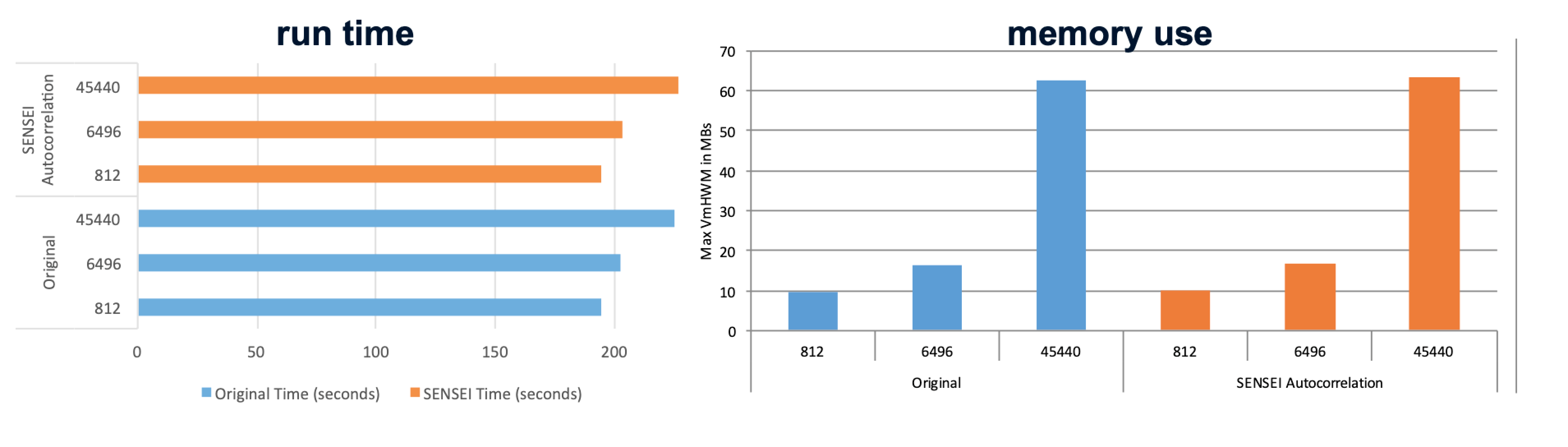
http://hpcvis.com/vis/sensei/rtd-docs/images/overheads.png

Run-time (left) and memory use (right) with (orange) and without (blue) SENSEI.

The full details of the performance and scaling studies can be found in our SC16 paper.

Analysis back-ends¶

Ascent back-end¶

Ascent is a many-core capable lightweight in-situ visualization and analysis infrastructure for multi-physics HPC simulations. The SENSEI AscentAnalysisAdaptor enables simulations instrumented with SENSEI to process data using Ascent.

SENSEI XML¶

The ascent back-end is activated using the <analysis type="ascent">. The supported attributes are:

attribute	description
actions	Path to ascent specific JSON file configuring ascent
options	Path to ascent specific JSON file configuring ascent

Back-end specific configurarion¶

SENSEI uses XML to select the specific back-end, in this case Ascent. The SENSEI XML will also contain references to Ascent specific configuration files that tell Ascent what to do. These files are native to Ascent. More information about configuring Ascent can be found in the Ascent documentation at https://ascent.readthedocs.io/en/latest/

Examples¶

Reaction rate in situ demo Ascent in situ demo.

Catalyst back-end¶

ParaView Catalyst (Catalyst) is an in situ use case library, with an adaptable application programming interface (API), that orchestrates the delicate alliance between simulation and analysis and/or visualization tasks. It brings the renown, scaling capabilities of VTK and ParaView to bear on the in situ use case. The analysis and visualization tasks can be implemented in C++ or Python, and Python scripts can be crafted from scratch or using the ParaView GUI to interactively setup Catalyst scripts (see Catalyst User Guide).

SENSEI XML Options¶

The Catalyst back-end is activated using the <analysis type="catalyst">.

Python Script¶

The supported attributes are:

attribute	description
pipeline	Use “pythonscript”.
filename	pythonscript filename.
enabled	“1” enables this back-end.

Example XML¶

Catalyst Python script example. This XML configures a Catalyst with a Python script that creates a pipeline(s).

<sensei>
<analysis type="catalyst" pipeline="pythonscript"
          filename="configs/random_2d_64_catalyst.py" enabled="1" />
</sensei>

Back-end specific configuration¶

The easiest way to create a python script for Catalyst:

Load a sample of the data (possibly downsampled) into ParaView, including all the desired fields.
Create analysis and visualization pipeline(s) in ParaView by applying successive filters producing subsetted or alternative visual metaphors of data.
Define a Catalyst extracts with the menu choice Catalyst→Define Exports: this will pop up the Catalyst Export Inspector panel.
Export the Catalyst Python script using the menu Catalyst→Export Catalyst Script.

The Catalyst Export Inspector reference.

Slice Fixed Pipeline¶

For the Catalyst slice fixed pipeline the supported attributes are:

attribute	description
pipeline	Use “slice”.
mesh	The name of the mesh to slice.
array	The data array name for coloring.
association	Either “cell” or “point” data.
image-filename	The filename template to write images.
image-width	The image width in pixels.
image-height	The image height in pixels.
slice-origin	The origin to use for slicing (optional).
slice-normal	The normal to use for slicing.
color-range	The color range of the array (optional).
color-log	Use logarithmic color scale (optional).
enabled	“1” enables this back-end

Example XML¶

This XML configures a C++-based fixed pipeline for a slice using Catalyst.

<sensei>
  <analysis type="catalyst"
            pipeline="slice" mesh="mesh" array="data" association="cell"
            image-filename="slice-%ts.png" image-width="1920" image-height="1080"
            slice-normal="0,0,1"
            color-range="0.0001,1.5" color-log="1"
            enabled="1" />
</sensei>

Particles Fixed Pipeline¶

For the Catalyst particle fixed pipeline the supported attributes are:

attribute	description
pipeline	Use “particle”.
mesh	The name of the mesh to slice.
array	The data array name for coloring.
association	Either “cell” or “point” data.
image-filename	The filename template to write images.
image-width	The image width in pixels.
image-height	The image height in pixels.
particle-style	The representation such as: “Gaussian Blur”, “Sphere”,
	“Black-edged circle”, “Plain circle”, “Triangle”, and
	“Square Outline”.
particle-radius	The normal to use for slicing.
color-range	The color range of the array (optional).
camera-position	The position of the camera (optional).
camera-focus	Where the camera points (optional).
enabled	“1” enables this back-end

Example XML¶

This XML configures a C++-based fixed pipeline for particles using Catalyst.

<sensei>
  <analysis type="catalyst"
     pipeline="particle" mesh="particles" array="data" association="point"
     image-filename="/tmp/particles-%ts.png" image-width="1920" image-height="1080"
     particle-style="Black-edged circle" particle-radius="0.5"
     color-range="0.0,1024.0" color-log="0"
     camera-position="150,150,100" camera-focus="0,0,0"
     enabled="1" />
</sensei>

Example¶

Reaction rate in situ demo ParaView Catalyst in situ demo.

Histogram back-end¶

As a simple analysis routine, the Histogram back-end computes the histogram of the data. At any given time step, the processes perform two reductions to determine the minimum and maximum values on the mesh. Each processor divides the range into the prescribed number of bins and fills the histogram of its local data. The histograms are reduced to the root process. The only extra storage required is proportional to the number of bins in the histogram.

SENSEI XML¶

The Histogram back-end is activated using the <analysis type="histogram">. The supported attributes are:

attribute	description
mesh	The name of the mesh for histogram.
array	The data array name for histogram.
association	Either “cell” or “point” data.
file	The filename template to write images.
bins	The number of histogram bins.

Example XML¶

Histogram example. This XML configures Histogram analysis.

<sensei>
  <analysis type="histogram"
    mesh="mesh" array="data" association="cell"
    file="hist.txt" bins="10"
    enabled="1" />
</sensei>

Back-end specific configurarion¶

No special back-end configuration is necessary.

Examples¶

VM Demo reference.

Autocorrelation back-end¶

As a prototypical time-dependent analysis routine, the Autocorrelation back-end computes the autocorrelation. Given a signal f(x) and a delay t, we find

\[\sum_{x}f(x)f(x+t).\]

Starting with an integer time delay t, we maintain in a circular buffer, for each grid cell, a window of values of the last t time steps. We also maintain a window of running correlations for each t′ ≤ t. When called, the analysis updates the autocorrelations and the circular buffer. When the execution completes, all processes perform a global reduction to determine the top k autocorrelations for each delay t′ ≤ t (k is specified by the user). For periodic oscillators, this reduction identifies the centers of the oscillators.

SENSEI XML¶

The Autocorrelation back-end is activated using the <analysis type="autocorrelation">. The supported attributes are:

attribute	description
mesh	The name of the mesh for autocorrelation.
array	The data array name for autocorrelation.
association	Either “cell” or “point” data.
window	The delay (t) for f(x).
k-max	The number of strongest autocorrelations to report.

Example XML¶

Autocorrelation example. This XML configures Autocorrelation analysis.

<sensei>
  <analysis type="autocorrelation"
    mesh="mesh" array="data" association="cell"
    window="10" k-max="3" enabled="1" />
</sensei>

Examples¶

VM Demo reference.

In transit transport layers and I/O¶

In transit data adaptor & control API¶

ADIOS-1¶

(Burlen)

ADIOS-2¶

(J.Logan)

Libis¶

(Silvio)

Data elevators¶

(Junmin)

Partitioners¶

The SENSEI end-point¶

Miniapps¶

oscillator¶

The oscillator mini-application computes a sum of damped, decaying, or periodic oscillators, convolved with (unnormalized) Gaussians, on a grid. It could be configured as a proxy for simulation of a chemical reaction on a two-dimensional substrate (see Chemical reaction on a 2D substrate).

option	description
-b, –blocks INT	Number of blocks to use [default: 1].
-s, –shape POINT	Number of cells in the domain [default: 64 64 64].
-e, –bounds FLOAT	Bounds of the Domain [default: {0,-1,0,-1,0,-1]}.
-t, –dt FLOAT	The time step [default: 0.01].
-f, –config STRING	SENSEI analysis configuration xml (required).
-g, –ghost-cells INT	Number of ghost cells [default: 1].
–t-end FLOAT	Request synchronize after each time step.
-j, –jobs INT	Number of threads [default: 1].
-o, –output STRING	Prefix for output [default: “”].
-p, –particles INT	Number of particles [default: 0].
-v, –v-scale FLOAT	Gradient to Velocity scale factor [default: 50].
-r, –seed INT	Random seed [default: 1].
–sync	The end time [default: 10].
-h, –help	Show help.

The oscillators’ locations and parameters are specified in an input file (see input folder for examples).

Note that the generate_input script can generate a set of randomly initialized oscillators.

The simulation code is in main.cpp while the computational kernel is in Oscillator.cpp.

To run:

There are a number of examples available in the SENSEI repositoory that leverage the oscillator mini-application.

newton¶

mandelbrot¶

Examples¶

Chemical reaction on a 2D substrate¶

This example illustrates how to select different back-ends at run time via XML, and how to switch in between in situ mode where the analysis runs in the same address space as the simulation and in transit mode where the analysis runs in a separate application called an end-point potentially on a different number of MPI ranks.

This example makes use of the oscillator mini-app configured as a proxy for simulation of a chemical reaction on a 2D substrate. The example uses different back-ends to make a pseudo coloring of the reaction rate with an iso-contour of 1. The Python analysis computes the area of the substrate where the reaction rate is greater or equal to 1 and plots it over time.

In situ demos¶

In this part of the demo XML files are used to switch back-end data consumer. The back-end data consumers are running in the same process as the simulation. This enables the use of zero-copy data transfer between the simulation and data consumer.

Ascent in situ demo¶

http://hpcvis.com/vis/sensei/rtd-docs/images/random_2d_64_ascent_00020.png

A pseudocolor plot rendered by Ascent of the rectaion rate field with an iso-contour plotted at a reaction rate of 1.0.

In the demo data from the reaction rate proxy simulation is processed using Ascent. Ascent is selected at run time via the following SENSEI XML:

<sensei>
  <analysis type="ascent" actions="configs/random_2d_64_ascent.json" enabled="1" >
    <mesh name="mesh">
        <cell_arrays> data </cell_arrays>
    </mesh>
  </analysis>
</sensei>

XML to select the Ascent back-end and configure it using a Ascent JSON
configuration

The analysis element selects Ascent, the actions attribute points to the Ascent specific configuration. In this case a JSON configuration. The following shell script runs the demo on the VM.

#!/bin/bash

n=4
b=64
dt=0.25
bld=`echo -e '\e[1m'`
red=`echo -e '\e[31m'`
grn=`echo -e '\e[32m'`
blu=`echo -e '\e[36m'`
wht=`echo -e '\e[0m'`

echo "+ module load sensei/3.1.0-ascent-shared"
module load sensei/3.1.0-ascent-shared

set -x

export OMP_NUM_THREADS=1

cat ./configs/random_2d_${b}_ascent.xml | sed "s/.*/$blu&$wht/"

mpiexec -n ${n} \
    oscillator -b ${n} -t ${dt} -s ${b},${b},1 -g 1 -p 0 \
    -f ./configs/random_2d_${b}_ascent.xml \
    ./configs/random_2d_${b}.osc 2>&1 | sed "s/.*/$red&$wht/"

During the run Ascent is configured to render a pseudocolor plot of the reaction rate field. The plot includes an iso-contour where the reaction rate is 1.

ParaView Catalyst in situ demo¶

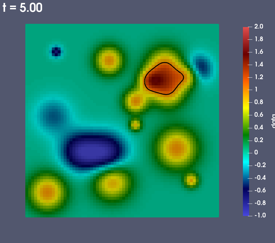
http://hpcvis.com/vis/sensei/rtd-docs/images/random_2d_64_catalyst_00020.png

A pseudocolor plot rendered by ParaView Catalyst of the rectaion rate field with an iso-contour plotted at a reaction rate of 1.0.

In the demo data from the reaction rate proxy simulation is processed using ParaView Catalyst. Catalyst is selected at run time via the following SENSEI XML:

<sensei>
  <analysis type="catalyst" pipeline="pythonscript"
    filename="configs/random_2d_64_catalyst.py" enabled="1" />
</sensei>

The analysis element selects ParaView Catalyst, the filename attribute points to the Catalyst specific configuration. In this case a Python script that was generated using the ParaView GUI. The following shell script runs the demo on the VM.

#!/bin/bash

n=4
b=64
dt=0.25
bld=`echo -e '\e[1m'`
red=`echo -e '\e[31m'`
grn=`echo -e '\e[32m'`
blu=`echo -e '\e[36m'`
wht=`echo -e '\e[0m'`

echo "+ module load sensei/3.0.0-catalyst-shared"
module load sensei/3.0.0-catalyst-shared

set -x

cat ./configs/random_2d_${b}_catalyst.xml | sed "s/.*/$blu&$wht/"

mpiexec -n ${n} \
    oscillator -b ${n} -t ${dt} -s ${b},${b},1 -g 1 -p 0 \
    -f ./configs/random_2d_${b}_catalyst.xml \
    ./configs/random_2d_${b}.osc 2>&1 | sed "s/.*/$red&$wht/"

During the run ParaView Catalyst is configured to render a pseudocolor plot of the reaction rate field. The plot includes an iso-contour where the reaction rate is 1.

VisIt Libsim in situ demo¶

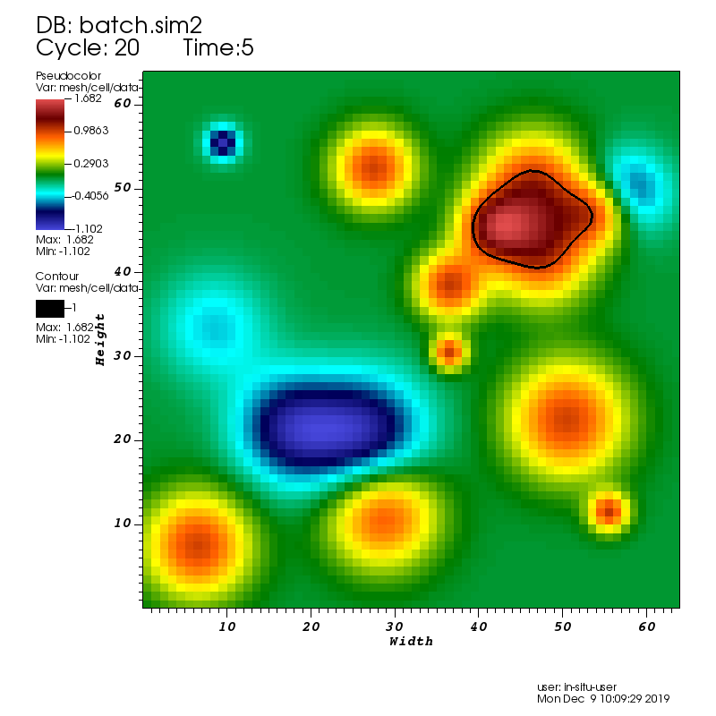
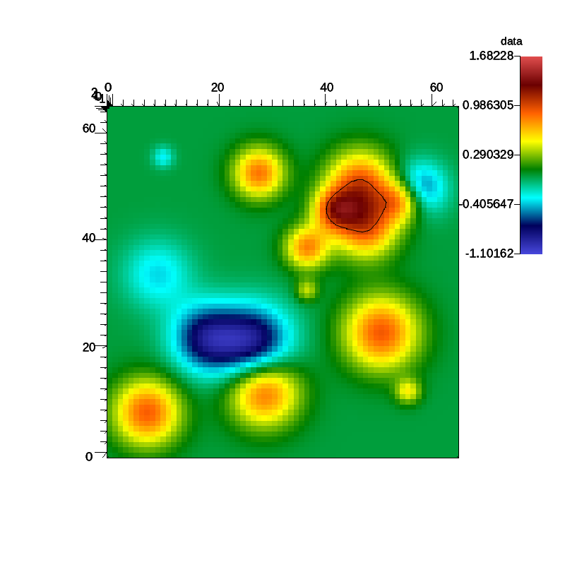
http://hpcvis.com/vis/sensei/rtd-docs/images/random_2d_64_libsim_00020.png

A pseudocolor plot rendered by VisIt Libsim of the rectaion rate field with an iso-contour plotted at a reaction rate of 1.0.

In the demo data from the reaction rate proxy simulation is processed using VisIt Libsim. Libsim is selected at run time via the following SENSEI XML:

<sensei>
  <analysis type="libsim" mode="batch" frequency="1"
            session="configs/random_2d_64_libsim.session"
            image-filename="random_2d_64_libsim_%ts"
            image-width="800" image-height="800" image-format="png"
            options="-debug 0" enabled="1" />
</sensei>

The analysis element selects VisIt Libsim, the filename attribute points to the Libsim specific configuration. In this case a session file that was generated using the VisIt GUI. The following shell script runs the demo on the VM.

#!/bin/bash

n=4
b=64
dt=0.25
bld=`echo -e '\e[1m'`
red=`echo -e '\e[31m'`
grn=`echo -e '\e[32m'`
blu=`echo -e '\e[36m'`
wht=`echo -e '\e[0m'`

echo "+ module load sensei/3.0.0-libsim-shared"
module load sensei/3.0.0-libsim-shared

set -x

cat ./configs/random_2d_${b}_libsim.xml | sed "s/.*/$blu&$wht/"

mpiexec -n ${n} \
    oscillator -b ${n} -t ${dt} -s ${b},${b},1 -g 1 -p 0 \
    -f ./configs/random_2d_${b}_libsim.xml \
    ./configs/random_2d_${b}.osc 2>&1 | sed "s/.*/$red&$wht/"

Shell script that runs the Libsim in situ demo on the VM.

During the run VisIt Libsim is configured to render a pseudocolor plot of the reaction rate field. The plot includes an iso-contour where the reaction rate is 1.

Python in situ demo¶

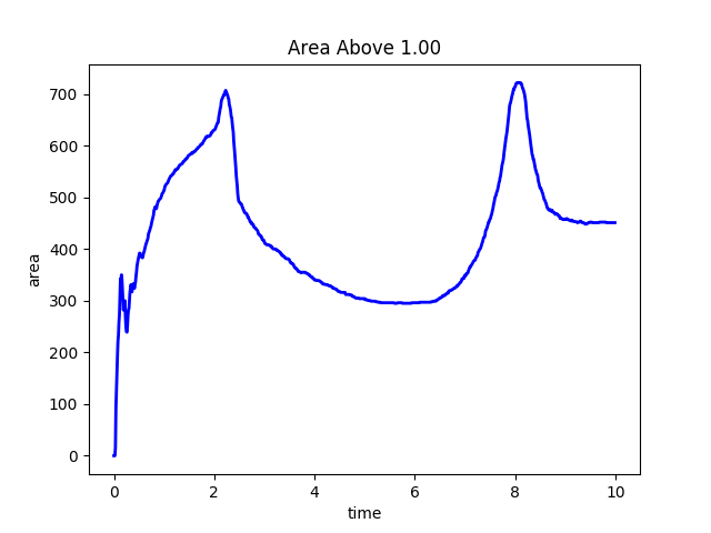
http://hpcvis.com/vis/sensei/rtd-docs/images/random_2d_64_python.png

A plot of the time history of the area of the 2D substrate where the reaction rate is greater or equal to 1.0.

In the demo data from the reaction rate proxy simulation is processed using Python. Python is selected at run time via the following SENSEI XML:

<sensei>
  <analysis type="python" script_file="configs/volume_above_sm.py" enabled="1">
    <initialize_source>
threshold=1.0
mesh='mesh'
array='data'
cen=1
out_file='random_2d_64_python.png'
     </initialize_source>
  </analysis>
</sensei>

The analysis element selects Python, the script_file attribute points to the user provided Python script and initialize_source contains run time configuration. The following shell script runs the demo on the VM.

#!/bin/bash

n=4
b=64
dt=0.01
bld=`echo -e '\e[1m'`
red=`echo -e '\e[31m'`
grn=`echo -e '\e[32m'`
blu=`echo -e '\e[36m'`
wht=`echo -e '\e[0m'`

export MPLBACKEND=Agg

echo "+ module load sensei/3.0.0-vtk-shared"
module load sensei/3.0.0-vtk-shared

set -x

cat ./configs/random_2d_${b}_python.xml | sed "s/.*/$blu&$wht/"

mpiexec -n ${n} oscillator -b ${n} -t ${dt} -s ${b},${b},1 -p 0 \
    -f ./configs/random_2d_${b}_python.xml \
    ./configs/random_2d_${b}.osc  2>&1 | sed "s/.*/$red&$wht/"

During the run this user provided Python script computes the area of the 2D substrate where the reaction rate is greater or equal to 1. The value is stored and at the end of the run a plot of the time history is made.

In transit demos¶

ParaView Catalyst¶

VisIt Libsim¶

Ascent¶

Python¶

Developer Guidelines¶

Git workflow¶

When working on a feature for a future release make a pull request targeting the develop branch. Only features to be included in the next release should be merged. A code review should be made prior to merge. New features should always be accompanied with read the docs documentation and at least one regression test.

We use the branching model described here: https://nvie.com/posts/a-successful-git-branching-model/ and detailed below in case the above link goes away in the future.

The main branches¶

The central repo holds two main branches with an infinite lifetime:

master
develop

The master branch at origin should be familiar to every Git user. Parallel to the master branch, another branch exists called develop.

We consider origin/master to be the main branch where the source code of HEAD always reflects a production-ready state.

We consider origin/develop to be the main branch where the source code of HEAD always reflects a state with the latest delivered development changes for the next release. Some would call this the “integration branch”.

When the source code in the develop branch reaches a stable point and is ready to be released, all of the changes should be merged back into master somehow and then tagged with a release number. How this is done in detail will be discussed further on.

Therefore, each time when changes are merged back into master, this is a new production release by definition. We tend to be very strict at this, so that theoretically, we could use a Git hook script to automatically build and roll-out our software to our production servers every time there was a commit on master.

Feature branches¶

May branch off from: develop Must merge back into: develop Branch naming convention: anything except master, develop, or release-*

Feature branches (or sometimes called topic branches) are used to develop new features for the upcoming or a distant future release. When starting development of a feature, the target release in which this feature will be incorporated may well be unknown at that point. The essence of a feature branch is that it exists as long as the feature is in development, but will eventually be merged back into develop (to definitely add the new feature to the upcoming release) or discarded (in case of a disappointing experiment).

Creating a feature branch¶

When starting work on a new feature, branch off from the develop branch.

$ git checkout -b myfeature develop

Incorporating a finished feature on develop¶

Finished features may be merged into the develop branch to definitely add them to the upcoming release:

$ git checkout develop
$ git merge --no-ff myfeature
$ git branch -d myfeature
$ git push origin develop

The –no-ff flag causes the merge to always create a new commit object, even if the merge could be performed with a fast-forward. This avoids losing information about the historical existence of a feature branch and groups together all commits that together added the feature.

Release branches¶

May branch off from: develop Must merge back into: develop and master Branch naming convention: release-*

Release branches support preparation of a new production release. They allow for last-minute dotting of i’s and crossing t’s. Furthermore, they allow for minor bug fixes and preparing meta-data for a release (version number, build dates, etc.). By doing all of this work on a release branch, the develop branch is cleared to receive features for the next big release.

The key moment to branch off a new release branch from develop is when develop (almost) reflects the desired state of the new release. At least all features that are targeted for the release-to-be-built must be merged in to develop at this point in time. All features targeted at future releases may not—they must wait until after the release branch is branched off.

It is exactly at the start of a release branch that the upcoming release gets assigned a version number—not any earlier. Up until that moment, the develop branch reflected changes for the “next release”, but it is unclear whether that “next release” will eventually become 0.3 or 1.0, until the release branch is started. That decision is made on the start of the release branch and is carried out by the project’s rules on version number bumping.

Creating a release branch¶

Release branches are created from the develop branch. For example, say version 1.1.5 is the current production release and we have a big release coming up. The state of develop is ready for the “next release” and we have decided that this will become version 1.2 (rather than 1.1.6 or 2.0). So we branch off and give the release branch a name reflecting the new version number:

$ git checkout -b release-1.2 develop
$ ./bump-version.sh 1.2
$ git commit -a -m "Bumped version number to 1.2"

After creating a new branch and switching to it, we bump the version number. Here, bump-version.sh is a fictional shell script that changes some files in the working copy to reflect the new version. (This can of course be a manual change—the point being that some files change.) Then, the bumped version number is committed.

This new branch may exist there for a while, until the release may be rolled out definitely. During that time, bug fixes may be applied in this branch (rather than on the develop branch). Adding large new features here is strictly prohibited. They must be merged into develop, and therefore, wait for the next big release.

Finishing a release branch¶

When the state of the release branch is ready to become a real release, some actions need to be carried out. First, the release branch is merged into master (since every commit on master is a new release by definition, remember). Next, that commit on master must be tagged for easy future reference to this historical version. Finally, the changes made on the release branch need to be merged back into develop, so that future releases also contain these bug fixes.

$ git checkout master
$ git merge --no-ff release-1.2
$ git tag -a 1.2

The release is now done, and tagged for future reference.

Code style¶

Here are some of the guidelines

use 2 spaces for indentation, no tabs or trailing white space
use CamelCase for names
variable names should be descriptive, with in reason
class member variables, methods, and namespace functions start with an upper case character, free functions start with a lower case
use the this pointer to access class member variables and methods
generally operators should be separated from operands by a single white space
for loop and conditional braces are indented 2 spaces, and the contained code is written at the same indentation level as the braces
functions and class braces are not indented, but contained code is indented 2 spaces.
a comment containing one space and 77 - precede class method definitions
pointers and reference markers should be preceded by a space.
generally wrap code at 80 chars
treat warnings as errors, compile with -Wall and clean all warnings
avoid 1 line conditionals

there are surely other details to this style, but I think that is the crux of it.

and a snippet to illustrate:

// a free function
void fooBar()
{
  printf("blah");
}

// a namespace
namespace myNs
{
// with a function
void Foo()
{
  pritf("Foo");
}

}

// a class
class Foo
{
public:
  // CamelCase methods and members
  void SetBar(int bar);
  int GetBar();

  // pointer and reference arguments
  void GetBar(int &bar);
  void GetBar(int *bar);

private:
  int Bar;
};

// ---------------------------------------------------------------------------
void Foo::SetBar(int bar)
{
  // a member function
  this->Bar = bar;
}

// ---------------------------------------------------------------------------
int Foo::GetBar()
{
  return this->Bar;
}

int main(int argc, char **argv)
{
  // a conditional
  if (strcmp("foo", argv[1]) == 0)
    {
    foo();
    }
  else
    {
    bar();
    }
  return 0;
}

Regressions tests¶

New classes should be submitted with a regression test.

User guide code style¶

Please use this style https://documentation-style-guide-sphinx.readthedocs.io/en/latest/style-guide.html

Glossary¶

List of all terms we defined