Examples

Chemical reaction on a 2D substrate

This example illustrates how to select different back-ends at run time via XML, and how to switch in between in situ mode where the analysis runs in the same address space as the simulation and in transit mode where the analysis runs in a separate application called an end-point potentially on a different number of MPI ranks.

This example makes use of the oscillator mini-app configured as a proxy for simulation of a chemical reaction on a 2D substrate. The example uses different back-ends to make a pseudo coloring of the reaction rate with an iso-contour of 1. The Python analysis computes the area of the substrate where the reaction rate is greater or equal to 1 and plots it over time.

In situ demos

In this part of the demo XML files are used to switch back-end data consumer. The back-end data consumers are running in the same process as the simulation. This enables the use of zero-copy data transfer between the simulation and data consumer.

Ascent in situ demo

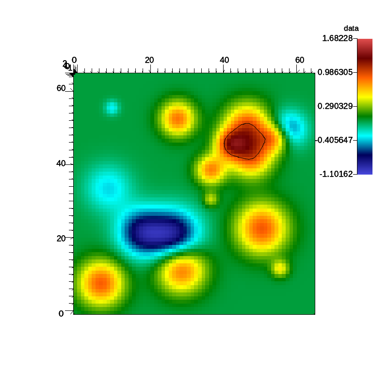
Fig. 7 A pseudocolor plot rendered by Ascent of the rectaion rate field with an iso-contour plotted at a reaction rate of 1.0.

In the demo data from the reaction rate proxy simulation is processed using Ascent. Ascent is selected at run time via the following SENSEI XML:

<sensei>
  <analysis type="ascent" actions="configs/random_2d_64_ascent.json" enabled="1" >
    <mesh name="mesh">
        <cell_arrays> data </cell_arrays>
    </mesh>
  </analysis>
</sensei>

XML to select the Ascent back-end and configure it using a Ascent JSON
configuration

The analysis element selects Ascent, the actions attribute points to the Ascent specific configuration. In this case a JSON configuration. The following shell script runs the demo on the VM.

#!/bin/bash

n=4
b=64
dt=0.25
bld=`echo -e '\e[1m'`
red=`echo -e '\e[31m'`
grn=`echo -e '\e[32m'`
blu=`echo -e '\e[36m'`
wht=`echo -e '\e[0m'`

echo "+ module load sensei/3.1.0-ascent-shared"
module load sensei/3.1.0-ascent-shared

set -x

export OMP_NUM_THREADS=1

cat ./configs/random_2d_${b}_ascent.xml | sed "s/.*/$blu&$wht/"

mpiexec -n ${n} \
    oscillator -b ${n} -t ${dt} -s ${b},${b},1 -g 1 -p 0 \
    -f ./configs/random_2d_${b}_ascent.xml \
    ./configs/random_2d_${b}.osc 2>&1 | sed "s/.*/$red&$wht/"

During the run Ascent is configured to render a pseudocolor plot of the reaction rate field. The plot includes an iso-contour where the reaction rate is 1.

ParaView Catalyst in situ demo

Fig. 8 A pseudocolor plot rendered by ParaView Catalyst of the rectaion rate field with an iso-contour plotted at a reaction rate of 1.0.

In the demo data from the reaction rate proxy simulation is processed using ParaView Catalyst. Catalyst is selected at run time via the following SENSEI XML:

<sensei>
  <analysis type="catalyst" pipeline="pythonscript"
    filename="configs/random_2d_64_catalyst.py" enabled="1" />
</sensei>

The analysis element selects ParaView Catalyst, the filename attribute points to the Catalyst specific configuration. In this case a Python script that was generated using the ParaView GUI. The following shell script runs the demo on the VM.

#!/bin/bash

n=4
b=64
dt=0.25
bld=`echo -e '\e[1m'`
red=`echo -e '\e[31m'`
grn=`echo -e '\e[32m'`
blu=`echo -e '\e[36m'`
wht=`echo -e '\e[0m'`

echo "+ module load sensei/3.0.0-catalyst-shared"
module load sensei/3.0.0-catalyst-shared

set -x

cat ./configs/random_2d_${b}_catalyst.xml | sed "s/.*/$blu&$wht/"

mpiexec -n ${n} \
    oscillator -b ${n} -t ${dt} -s ${b},${b},1 -g 1 -p 0 \
    -f ./configs/random_2d_${b}_catalyst.xml \
    ./configs/random_2d_${b}.osc 2>&1 | sed "s/.*/$red&$wht/"

During the run ParaView Catalyst is configured to render a pseudocolor plot of the reaction rate field. The plot includes an iso-contour where the reaction rate is 1.

VisIt Libsim in situ demo

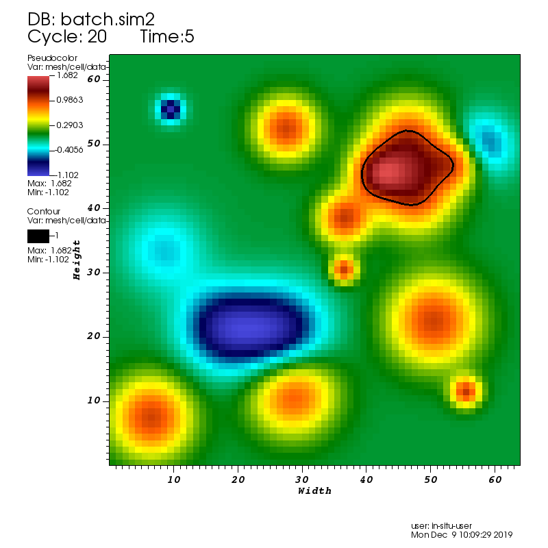
Fig. 9 A pseudocolor plot rendered by VisIt Libsim of the rectaion rate field with an iso-contour plotted at a reaction rate of 1.0.

In the demo data from the reaction rate proxy simulation is processed using VisIt Libsim. Libsim is selected at run time via the following SENSEI XML:

<sensei>
  <analysis type="libsim" mode="batch" frequency="1"
            session="configs/random_2d_64_libsim.session"
            image-filename="random_2d_64_libsim_%ts"
            image-width="800" image-height="800" image-format="png"
            options="-debug 0" enabled="1" />
</sensei>

The analysis element selects VisIt Libsim, the filename attribute points to the Libsim specific configuration. In this case a session file that was generated using the VisIt GUI. The following shell script runs the demo on the VM.

#!/bin/bash

n=4
b=64
dt=0.25
bld=`echo -e '\e[1m'`
red=`echo -e '\e[31m'`
grn=`echo -e '\e[32m'`
blu=`echo -e '\e[36m'`
wht=`echo -e '\e[0m'`

echo "+ module load sensei/3.0.0-libsim-shared"
module load sensei/3.0.0-libsim-shared

set -x

cat ./configs/random_2d_${b}_libsim.xml | sed "s/.*/$blu&$wht/"

mpiexec -n ${n} \
    oscillator -b ${n} -t ${dt} -s ${b},${b},1 -g 1 -p 0 \
    -f ./configs/random_2d_${b}_libsim.xml \
    ./configs/random_2d_${b}.osc 2>&1 | sed "s/.*/$red&$wht/"

Shell script that runs the Libsim in situ demo on the VM.

During the run VisIt Libsim is configured to render a pseudocolor plot of the reaction rate field. The plot includes an iso-contour where the reaction rate is 1.

Python in situ demo

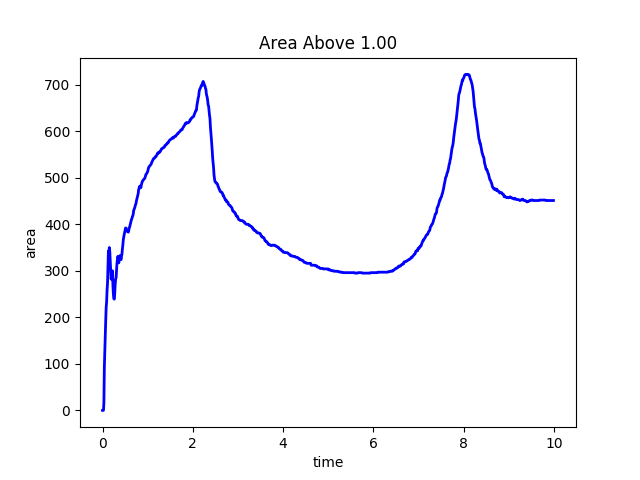
Fig. 10 A plot of the time history of the area of the 2D substrate where the reaction rate is greater or equal to 1.0.

In the demo data from the reaction rate proxy simulation is processed using Python. Python is selected at run time via the following SENSEI XML:

<sensei>
  <analysis type="python" script_file="configs/volume_above_sm.py" enabled="1">
    <initialize_source>
threshold=1.0
mesh='mesh'
array='data'
cen=1
out_file='random_2d_64_python.png'
     </initialize_source>
  </analysis>
</sensei>

The analysis element selects Python, the script_file attribute points to the user provided Python script and initialize_source contains run time configuration. The following shell script runs the demo on the VM.

#!/bin/bash

n=4
b=64
dt=0.01
bld=`echo -e '\e[1m'`
red=`echo -e '\e[31m'`
grn=`echo -e '\e[32m'`
blu=`echo -e '\e[36m'`
wht=`echo -e '\e[0m'`

export MPLBACKEND=Agg

echo "+ module load sensei/3.0.0-vtk-shared"
module load sensei/3.0.0-vtk-shared

set -x

cat ./configs/random_2d_${b}_python.xml | sed "s/.*/$blu&$wht/"

mpiexec -n ${n} oscillator -b ${n} -t ${dt} -s ${b},${b},1 -p 0 \
    -f ./configs/random_2d_${b}_python.xml \
    ./configs/random_2d_${b}.osc  2>&1 | sed "s/.*/$red&$wht/"

During the run this user provided Python script computes the area of the 2D substrate where the reaction rate is greater or equal to 1. The value is stored and at the end of the run a plot of the time history is made.

In transit demos

ParaView Catalyst

VisIt Libsim

Ascent

Python

Building Pipelines

Pipelines of in situ and in transit operations can be constructed by chaining sensei::AnalysisAdaptors using C++ or Python.

The following example shows a SENSEI PythonAnalysis script that configures and executes a simple pipeline that calculates a set of iso-surfaces using SENSEI’s SliceExtract and then writes them to disk using SENSEI’s VTKPosthocIO analysis adaptor.

from sensei import SliceExtract, VTKPosthocIO
from svtk import svtkDataObject
import sys

# control
meshName  = None
arrayName  = None
arrayCen  = None
isoVals  = None
outputDir  = None

# state
slicer = None
writer = None

def Initialize():
    global slicer,writer
    if comm.Get_rank() == 0:
        sys.stderr.write('PipelineExample::Initialize\n')
        sys.stderr.write('meshName=%s, arrayName=%s, arrayCen=%d, '
                         'isoVals=%s, outputDir=%s\n'%(meshName,
                         arrayName, arrayCen, str(isoVals), outputDir))

    slicer = SliceExtract.New()
    slicer.EnableWriter(0)
    slicer.SetOperation(SliceExtract.OP_ISO_SURFACE)
    slicer.SetIsoValues(meshName, arrayName, arrayCen, isoVals)
    slicer.AddDataRequirement(meshName, arrayCen, [arrayName])

    writer = VTKPosthocIO.New()
    writer.SetGhostArrayName('ghosts')
    writer.SetOutputDir(outputDir)
    writer.SetWriter(VTKPosthocIO.WRITER_VTK_XML)
    writer.SetMode(VTKPosthocIO.MODE_PARAVIEW)

def Execute(daIn):
    if comm.Get_rank() == 0:
        sys.stderr.write('PipelineExample::Execute %d\n'%(daIn.GetDataTimeStep()))

    # stage 1 - iso surface
    isoOk, iso = slicer.Execute(daIn)

    if not isoOk:
        return 0

    # stage 2 - write the result
    writer.Execute(iso)

    return 1

def Finalize():
    if comm.Get_rank() == 0:
        sys.stderr.write('PipelineExample::Finalize\n')

    slicer.Finalize()
    writer.Finalize()

For the purposes of this demo, the above Python script is stored in a file named “iso_pipeline.py” and refered to in the XML used to configure the system. The XML used to configure the system to run the iso-surface and write pipeline is shown below:

<sensei>
  <analysis type="python" script_file="iso_pipeline.py" enabled="1">
    <initialize_source>
meshName = 'mesh'
arrayName = 'data'
arrayCen = svtkDataObject.CELL
isoVals = [-0.619028, -0.0739720000000001, 0.47108399999999995, 1.01614]
outputDir = 'oscillator_iso_pipeline_%s'%(meshName)
     </initialize_source>
  </analysis>
</sensei>

The variables meshName, arrayName, arrayCen, isoVals, and outputDir are used to configure for a specific simulation or run. For the purposes of this demo this XML is stored in a file name iso_pipeline.xml and passed to the SENSEI ConfigurableAnalaysis adaptor during SENSEI initialization.

One can run the above pipeline with the oscillator miniapp that ships with SENSEI using the following shell script.

#!/bin/bash

 module load mpi/mpich-x86_64
 module use /work/SENSEI/modulefiles/
 module load sensei-vtk

 mpiexec -np 4 oscillator -t .5 -b 4 -g 1 -f iso_pipeline.xml simple.osc